International Journal of Innovation and Economic Development

Volume 11, Issue 5, Dec 2025, Pages 21-35

---

Time series analysis of global temperature trends in the context of anthropogenic climate change

DOI: 10.18775/ijied.1849-7551-7020.2015.115.2002
URL: https://doi.org/10.18775/ijied.1849-7551-7020.2015.115.2002

Sven Birkenfeld ¹,  Arthur Dill, ¹

¹FOM University of Applied Science, Essen, Germany

Abstract: This study investigates the use of machine learning methods to predict global temperature anomalies in the context of anthropogenic climate change. The research uses a comprehensive dataset comprising historical temperature records, greenhouse gas concentrations, sea level trends, and key atmospheric and oceanic indices to evaluate the predictive capabilities of three time series models (XGBoost, SVR, and LSTM). The dataset, compiled from several authoritative sources, underwent rigorous preprocessing, including imputation, interpolation, and correlation-based feature selection. The models were trained and validated using a time series cross-validation approach and evaluated using standard error metrics such as MAPE, RMSE, and MAE. Due to data limitations, the test dataset spans only about 2-3 years, so any assessment of long-term trends in model performance should be interpreted conceptually. Taking this into account, the LSTM network demonstrated the best forecast performance, especially in capturing long-term warming trends, while the SVR model showed comparable results with slightly lower precision. The XGBoost model showed a tendency to underperform, particularly in its ability to represent values at the extremes of the data distribution. Despite the limitations of the models in fully capturing short-term fluctuations or extreme anomalies, the results underscore the potential of deep learning approaches, particularly LSTM, for improving climate forecasts. The results of the study suggest that machine learning has the potential to be a valuable complement to traditional physical climate models but cannot completely replace them. The research suggests that machine learning models could be trained primarily with input and output data from established climate models in the future in order to quickly and efficiently reproduce the results of climate models and analyze various climate scenarios.

 

Keywords: anthropogenic climate change; time series analysis; global temperature prediction; machine learning; artificial intelligence

 

1. Introduction

Anthropogenic climate change has been documented for several decades. Between February 2023 and January 2024, the average temperature was 1.52 degrees above pre-industrial levels, representing a new record (Mayr, 2024).  The main causes of this development can be found in the areas of energy production, industry, agriculture, and transportation. These sectors constantly and increasingly produce greenhouse gases such as carbon dioxide, methane, and nitrous oxide, which accumulate in the atmosphere and contribute to global warming. If these emissions are not significantly reduced, global temperatures could change dramatically in a short period of time (Lehmann et al., 2013). This global warming has far-reaching and serious consequences that are already visible today and include extreme weather events such as forest fires, droughts, and heavy rainfall. In addition, famines and food crises are intensifying, as is the spread of infectious diseases. Climate change must therefore be addressed as one of the central challenges of the 21st century. In the Paris Agreement, the international community committed in 2015 to limit global warming to 1.5 to 2.0 degrees Celsius (Boetius et al., 2021). However, at the climate conference in Glasgow at the end of 2021, it was determined that the agreed targets had not been met and that the measures to reduce emissions would not be sufficient to limit the temperature increase within the agreed target (Dwivedi et al., 2022).  Instead, based on current climate projections, it can be assumed that without a reduction in greenhouse gas emissions, global warming of 0.2 degrees Celsius per decade is very likely over the next 30 years. Numerical climate models are primarily used to study future climate change, generating simulation results based on various emission scenarios (Umweltbundesamt, 2024). This work also aims to investigate the contribution that artificial intelligence can make to predicting future temperature increases. To this end, three specific time series models — the gradient boosting decision tree, support vector regression, and long short-term memory — are considered, and their performance in predicting global temperature deviations is evaluated.

 

 

1.1 Aim of the study

This paper addresses the problem of rising temperatures and their impacts on humanity and nature. Further, it aims to provide a machine-learning-based statistical time-series approach for predicting global temperature changes. To this end, various time series analysis techniques are used to examine historical climate data and identify patterns within it. In this context, an analysis using different time series models will serve to explore their specific strengths and weaknesses and ensure optimal results. This paper considers gradient boosting decision tree, support vector regression, and long short-term memory techniques as specific solutions. The development and evaluation of the models are intended to highlight which factors have a central influence on temperature change and which trends can be identified within these factors. Taking these characteristics into account, the study aims to provide a reliable forecast of future temperature changes. These considerations give rise to the following central research questions for this thesis:

• What long-term trends can be derived from historical temperature data?
• How effective are time series models in predicting global temperature changes caused by anthropogenic climate change?
• Which factors influence the accuracy of the forecast, and how significant is their respective influence?
• How do the time series models differ, and which is best suited to predict temperature trends?

 

 

2. Literature Review

In climate and weather research, there is a fundamental distinction between weather forecasting, climate forecasting, and climate projection. Weather forecasts predict short-term weather conditions and cover a period of a few hours to fourteen days at most. In contrast, climate forecasts provide an indication of long-term climate trends over a medium-term period. Within this category, further distinctions can be made between sub-seasonal forecasts (covering the next three to six weeks), seasonal forecasts (covering the next one to six months) and decadal climate forecasts (covering the next ten years). Furthermore, climate projections cover an even longer time horizon, typically extending to the end of the 21st century. The models created in this context are therefore primarily influenced by the greenhouse effect (Deutscher Wetterdienst, 2024a). Different scenarios for future social development are used to estimate future emission levels. At the same time, such a climate model encompasses all the essential processes of the Earth's atmosphere, biosphere, hydrosphere and cryosphere. These are considered subsystems of the climate system as a whole and are usually represented by their own computational models, which are later linked together to form the overall model. This makes climate models some of the most complex and computationally intensive models of our time (Deutscher Wetterdienst, 2024b). By contrast, machine learning methods rely solely on historical observational data and do not explicitly model the underlying physical processes of the climate system. This allows them to produce statistical time-series results, primarily for short-term forecasts, with much greater computational efficiency. The study by Bochenek et al. lends further support to this assumption and demonstrates that machine learning can play a significant role in future weather forecasting (Bochenek & Ustrnul, 2022). Zhu et al. utilise time series methodologies to analyse and evaluate temperature data. Furthermore, an ARIMA model is employed to predict the global average temperature until the year 2100 (Zhu & Li, 2023). In addition, there are also approaches that focus specifically on predicting the dynamics of future sea surface temperatures based on time series satellite data. Xiao et al. use a machine learning method that combines a deep recurrent neural network model with long short-term memory (LSTM) and an AdaBoost ensemble learning model. In this way, the strengths of the LSTM network in terms of modeling long-term dependencies can be combined with the robustness of AdaBoost against overfitting. A case study conducted in this context in the East China Sea, in which daily sea surface temperatures were predicted 10 days in advance, shows that the combined LSTM-AdaBoost model outperforms the individual LSTM and AdaBoost models, as well as a proven feedforward backpropagation neural network model (BPNN) and a support vector regression model (SVR) (Xiao et al., 2019).

 

This paper also aims to examine various machine learning approaches in order to evaluate their performance with regard to predictions of global temperature anomalies. The study evaluates and compares the performance of a support vector regression as well as an XGBoost and LSTM model. This approach helps identify each model's unique strengths and determine the most effective prediction method for this context.

 

 

3. Research Methodology

 

The dataset considered was compiled from various sources and contains key information on the causes and consequences of anthropogenic climate change. Key measurements of global temperature anomalies are taken from the NOAA Global Surface Temperature Dataset. These data combine sea and land surface temperatures and present them as global anomalies relative to the monthly climatology from 1971 to 2000. The specific data was retrieved in the form of monthly averages (Huang et al., 2024). In addition, further climate-related information was added to the dataset. This includes sea level, the atmospheric concentrations of specific greenhouse gases, the mass balance of reference glaciers, the sea ice concentration, and climatic phenomena such as the ENSO cycle and the North Atlantic Oscillation. Figure 1 summarises the data sources used and indicates the metrics in which observation values are available.

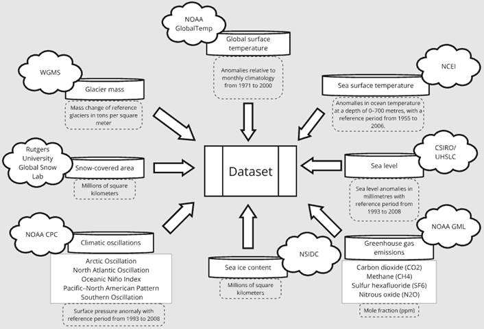
Figure 1: Overview of data sources and metrics

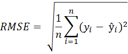
The development of time series models follows the Cross Industry Standard Process for Data Mining (CRISP-DM). To perform a qualitative assessment of the performance of the developed time series models, various evaluation metrics are used to quantify the difference between the model's predicted values and the actual values of the test data. These metrics are crucial as they indicate how well the model captures underlying temporal patterns and trends. Table 1 presents the evaluation metrics used and their formal definitions (Kolambe & Arora, 2024).

Table 1: Evaluation metrics and their formal representation

Evaluation metric	Formal definition
Mean Absolute Error (MAE)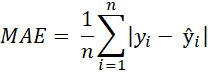
Mean Squared Error (MSE)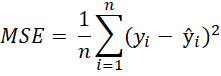
Root Mean Squared Error (RMSE)
Mean Absolute Percentage Error (MAPE)

4. Data Analysis and Interpretation

 

4.1. Data Understanding

An examination of the temperature anomalies reveals a clear increase since 1910. A particularly sharp increase is evident from 2010 onwards (Figure A1). Closer examination of the data from 1960 onward confirms this trend (Figure A2) (Huang et al., 2024). The available data also shows an increase in the greenhouse gas emissions under consideration in recent years (Figures A3-A6). Only methane levels stagnated between 1999 and 2005, but then also continued to rise. Sulfur hexafluoride levels have even more than doubled since 1998 (Lan et al., 2024). This is due to the fact that the greenhouse gas has been increasingly used industrially since 1960, primarily for insulation in energy transmission and distribution equipment. To date, sulfur hexafluoride has not contributed significantly to climate change. Nevertheless, it has a very high climate impact. Therefore, a sharp increase in the atmospheric concentration of this gas is not harmless, and measures are already being taken to reduce it (Wissenschaftliche Dienste - Deutscher Bundestag, 2022). The steady warming of the ocean has also been recorded since 1955 (Figure A7) (Lindsey & Dahlman, 2023). As a direct consequence of this warming, there has been a steady rise in sea levels (Figure A8) (Church & White, 2011) and a drastic decline in sea ice on both hemispheres (Figure A9) (Fetterer et al., 2017). However, it is not only sea ice that has been shrinking over the past years. Global glacier mass (Figure A10)  (Braithwaite & Hughes, 2020) and snow cover in the northern hemisphere (Figure A11) (Robinson et al., 2012) are also declining dramatically. Cyclical natural climate changes can also lead to seasonal fluctuations in temperature anomalies. These phenomena are influenced by various factors, including the fluctuations in air pressure in specific regions and the associated change in sea surface temperature (Lindsey, 2009a). In this context, the North Atlantic Oscillation Index, the Arctic Oscillation Index, the Southern Oscillation Index, and the Pacific-North America Index are particularly relevant. When taking the Southern Oscillation into account, it is also possible to draw conclusions about the occurrence of El Niños and La Niñas. These phenomena are closely linked to atmospheric circulation patterns in the southern Pacific. In this context, the ONI index is used to identify anomalies that reflect ENSO cycles (Lindsey, 2009b). Figure A12 clearly shows that these cycles can vary in strength and duration. Nevertheless, the individual phases can be clearly derived from past data. This assertion also pertains to the other climatic oscillations that are considered in the analysis (Figures A13-A17) (NOAA Climate Prediction Center, 2024).

 

4.2. Data Preparation

A thorough examination of the complete data set reveals the presence of missing observation values, which are subsequently imputed during the data preparation process. Notably, significant lacunae are evident within the dataset concerning snowfall, particularly during the interval from June to October 1969 and extending to several months in 1968 and 1971. A notable omission in the documentation is the absence of snowfall data during the warmer summer months. This omission introduces a distortion in the presentation of annual averages, as illustrated in Figure A18. To complete the observations, the data is therefore imputed using linear interpolation. These imputed data result in lower mean values for the years 1969 and 1971. However, compared to subsequent years, these are still considered to be years with higher snowfall (Figure A19). This observation is not implausible, as documented extreme weather events such as the “100-hour snowstorm” in February 1969 demonstrate that above-average snowfall was indeed recorded in that year (Squires, 2016).

 

For the data set under consideration, it should also be noted that the start date of the individual measurements may vary. When the data sets are merged, this results in missing values for periods that were not observed. Figure 2 presents a comprehensive overview of the periods during which observation values are available for the variables under examination.

 

Figure 2: Observation periods and intervals for the variables examined

 

It is evident that most of the data was collected at monthly intervals. The values for sea level, sea surface temperature, and glacier mass constitute exceptions to this general pattern. These are only available at quarterly or annual intervals. The combination of these data sets results in incomplete observations. Consequently, monthly values are incorporated in advance for these characteristics using linear interpolation. In contrast, the sea ice content of the northern and southern hemispheres is systematically monitored at more frequent intervals, with daily observations commencing in August 1987. To utilize monthly values when considering these variables, they are converted into corresponding mean values. In addition to the occurrence of missing values due to varying observation intervals, missing values resulting from a shorter observation period must also be considered. In this regard, the measured values of greenhouse gases are of particular interest. The CO₂ content in the atmosphere has been meticulously recorded since 1979. The measurement of atmospheric N₂O has only been conducted since 2001. The CH₄ and SF₆ content has also only been recorded for a few decades. For the columns under consideration, a linear regression of the data is therefore performed to obtain an estimate of their values before the initiation of the observation period. Figures A20-A23 illustrate the data values extrapolated in this way. In this context, the constant shown describes the start of the actual data collection. In general, the data is well supplemented by linear regression. However, it should be noted that prior to the initiation of data collection, there is a discernible tendency for more substantial implausible fluctuations in the mole fraction to manifest. But since the entire time series is being considered, these are regarded as negligible in the following. Furthermore, it should be noted that the generally low measured values of atmospheric SF₆ content, combined with the linear determination of the previous year's values, yield negative results across all years considered before 1998. Since negative emissions do not appear plausible for this period, such an imputation of values is not appropriate. Instead, the actual observations are logarithmically transformed in advance and then supplemented using linear regression. This approach results in the data shown in Figure A24. After the transformation of the data, the time series exhibits exponential growth. Given that the use of this greenhouse gas has been limited to industrial applications since 1960, this approach facilitates a more accurate representation of the increasing rise in atmospheric content. In addition to greenhouse gas emissions, data values for southern and northern sea ice content are also extrapolated using linear regression. The observed sea level values are supplemented beyond 2020 using exponential smoothing. Figure 3 shows the scope of all data preprocessing steps performed for the individual columns of the dataset. Data values are generally extrapolated for previous years up to 1950 and subsequent years up to 2024.

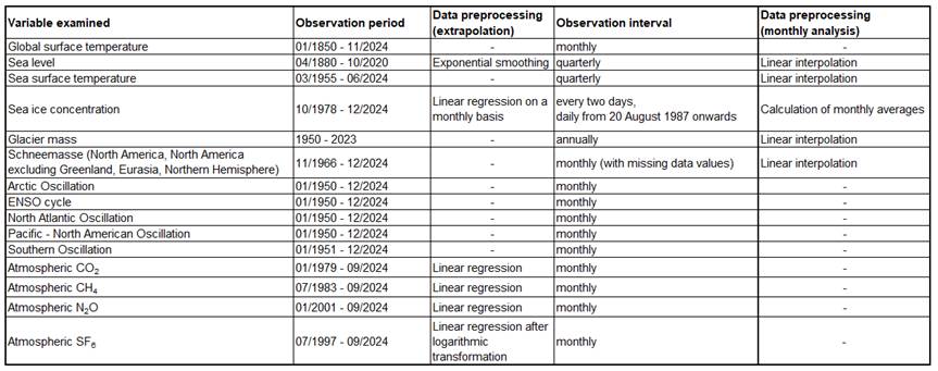
Figure 3: Data preprocessing of the variables examined

In this context, it is important to note that the used methods in data preprocessing enable the construction of a temporally consistent dataset but still represent simplified approximations of underlying physical processes, while the variables may exhibit nonlinear behaviour that is not fully captured by these approaches. Consequently, the so extrapolated and imputed values, especially for periods prior to the onset of systematic observations, are subject to increased uncertainty and should be interpreted as approximate estimates rather than exact physical reconstructions. Nevertheless, regression-based extrapolation is used instead of paleoclimatic reconstructions in order to maintain the temporal consistency of the data set and remain aligned with the statistical focus of the study.

 

The first day of each month is designated as the index date for the time series. The year associated with this date and the month under consideration are added to the data set as separate feature columns so that they can be included as additional independent variables during model training. Prior to the modeling phase, the complete dataset is also reduced to the period from January 1967 to December 2023. This approach is designed to minimize the use of imputed values during model training, thereby ensuring the integrity and reliability of the data.

4.3 Modeling and Evaluation

After data preprocessing, the final dataset comprises a total of 684 rows. Each of these rows contains 20 descriptive feature columns and the anomaly of the global surface temperature as the target variable. To forecast this target value, an extreme gradient boosting model, a support vector regression, and a long short-term memory network are employed. The neural network under consideration consists of an input layer, three LSTM layers, and an output layer. Each LSTM layer can be succeeded by a dropout layer, which is intended to prevent overfitting of the model. The number of neurons is reduced by half for each subsequent LSTM layer. Consequently, the third and final layer contains one-quarter of the neurons present in the first layer. The data is entered into the model in sequences of length five so that temporal patterns and dependencies are taken into account in model training. A rough overview of the architecture of the LSTM network is shown in Figure 4.

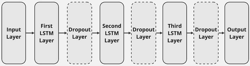
Figure 4: LSTM network architecture

 

For the SVR and XGBoost models, no explicit windowing was used, so these models were trained on the raw feature columns at each time step, and any temporal dependencies are implicitly captured from the sequential ordering of the data. This approach preserves the relative simplicity of these non-sequential models compared to the inherently more complex LSTM, as introducing lagged features or windowing would increase the models complexity and also the risk of overfitting without guaranteeing substantial benefit.

Before each model was trained with the data, the dimensionality and thus also the complexity of the dataset was reduced by identifying variables that have a high explanatory value in relation to the prediction of the target variables. To this end, the correlations were initially determined using Pearson's coefficient (Ly et al., 2018). The result of this correlation analysis is shown in Figure 5.

 

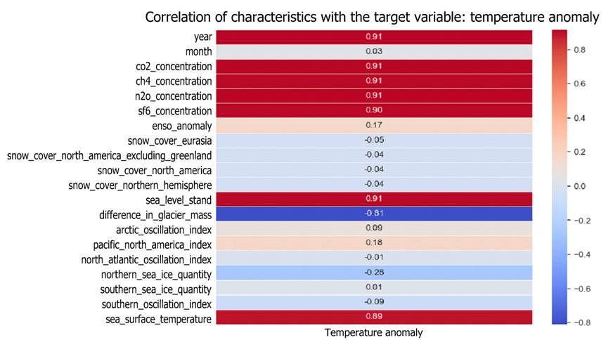
Figure 5: Correlation of feature columns and target variable

The characteristics identified in this process correspond to those variables that show the highest average gain in accuracy when training an initial XGBoost model (Figure 6) (Piraei et al., 2023).

Figure 6: Features with the highest “gain” - value

For this reason, before designing the final models, the data set is reduced to the 15 most relevant characteristics identified in this context. To enable subsequent validation of the results, the entire data set is also divided into three smaller sub-data sets. The largest of these data sets consists of 80% of the total observations and comprises the training data used to learn the structures and data patterns. Another 15% of the data set is used as validation data for optimizing the model. This ensures that the machine learning model developed has optimal parameters for the problem at hand. The remaining 5% of the data is used for final testing of the model (Burzykowski et al., 2023). The optimal model parameters are identified using grid search (Ramadhan et al., 2017). The parameters considered for each model are shown in Figure 7.

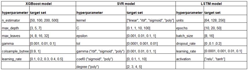
Figure 7: Hyperparameters and target sets considered

 

These hyperparameters are optimized based on a fivefold time series split. This allows validation using different test indices without changing the structure of the time series by randomly mixing the data rows (Pedregosa et al., 2011). The performance of the cross-validated models is measured using the root mean squared error. Since the predictive performance of SVR models is strongly influenced by the size and fluctuations within the input data, it also makes sense to normalize the data before training these models (Tran et al., 2022). As the individual characteristics do not contain any extraordinary outliers, the min-max normalization method is used in this paper. When dealing with this processing step, it is crucial to avoid data leakage. This problem arises when information from the test or validation data set unintentionally flows into the training of the model. Such leaks can cause the model to show unrealistically high performance, which cannot be transferred to unknown data (Bouke & Abdullah, 2023).  To prevent these undesirable effects, a data pipeline is used. This combines the steps of data transformation and model training and subjects them to cross-validation (Pedregosa et al., 2011). The results of the hyperparameter optimization performed are shown in Figure 8.

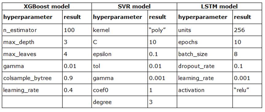
Figure 8: Results of hyperparameter optimization

To determine the optimal learning rate of the XGBoost model and the optimal C-value of the support vector regression with greater precision, these are examined in more detail in a subsequent step. To this end, the mean absolute percentage error of different models with varying learning rates and C-values is evaluated, with other parameters set according to the hyperparameter optimization. It should be noted that MAPE can be sensitive when target values are very small, as even minor absolute deviations may lead to relatively large percentage errors. In the present validation and test data, a few temperature anomalies are only slightly above zero, but no zero values occur outside of the train dataset. Therefore, while MAPE may slightly overemphasize errors for these small anomalies, it still provides a meaningful measure of relative performance, especially when interpreted together with absolute error metrics such as RMSE. Following the described procedure, the analysis yields an optimal learning rate of 0.34 and an optimal C-value of 20. After adjusting these parameters, the models achieve slightly better results, which are shown in Figure 9.

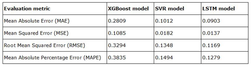
Figure 9: Results of the time series models on the test data

 

 

 

Figures 10-12 also show the entire time series and the predictions of the individual models based on the validation and test data.

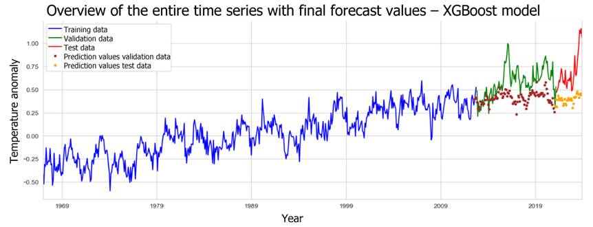
Figure 10: Forecast results from the XGBoost model for the whole time series.

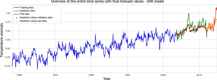
Figure 11: Forecast results from the SVR model for the whole time series.

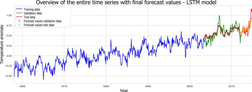
Figure 12: Forecast results from the LSTM model for the whole time series.

 

 

This comparison underlines that the LSTM model achieves the best result in terms of MAPE with 12.79%. The neural network also achieves the best results in terms of absolute values. The optimized SVR model performs only slightly worse overall. Conversely, the XGBoost model proves to be less powerful, achieving a MAPE that is approximately 25.5 percentage points higher than that of the neural network. Absolute error measures also show weaker results in this context. The distribution of the predicted values, as illustrated in Figure 13, underscores the limitations of the XGBoost model's forecasts.

Figure 13: Distribution of predicted and actual temperature deviations

 

 

Overall, none of the model predictions can ultimately reflect the high dispersion of actual temperature anomalies. On average, the SVR model's predictions are largely in line with the observed values. But the slight difference in the minimum and the substantial difference at the upper end show that the SVR model cannot accurately predict outliers in the test data. Long-term prognoses of temperature anomalies, considering specific socioeconomic assumptions, are therefore best made using the developed LSTM model, as it was already most effective at anticipating the short-term underlying increase in anomaly values in the test data.

 

 

5. Conclusion and Recommendations

Within this study, various time series models were used to forecast temperature trends. In this context, the performance of the XGBoost, SVR, and LSTM models was evaluated in relation to the problem at hand. These three time series models are based on different machine learning approaches: extreme gradient boosting, support vector machines and neural networks. The individual models were trained using a dataset compiled from various sources, which included a wide range of climate-related variables. Exploratory analysis of these characteristics revealed clear trends, which in many cases were accompanied by exponential growth. A correlation analysis of the variables showed a positive relationship between the atmospheric content of greenhouse gases and the observed temperature anomalies. This direct correlation was also confirmed during the training of the XGBoost model. In this context, the average information gain of the features during the decision tree splits was observed. Overall, the prediction results show that the basic trend of temperature anomalies can be correctly predicted. The optimized SVR and LSTM models in particular are able to anticipate future trends in the anomaly values. Only the predictions of the developed XGBoost model were unconvincing, as they were significantly lower than the actual observed values. It is also important to emphasise that none of the models were able to accurately predict short-term fluctuations in temperature anomalies. It is therefore also questionable whether possible sharp rises in temperature due to positive feedback loops, such as those seen in climate tipping elements, can be reliably captured by time series forecasts. However, a grid search carried out in the study shows that optimising the parameters can indeed lead to an increase in prediction accuracy. In this regard, a more extensive grid search could improve the final overall result of all models considered. An expansion of the data set is also conceivable. In this study, a time series with monthly data collection was examined. A more detailed analysis of data based on a shorter collection interval, which would provide a larger number of data points, could yield more precise and meaningful results. Neural networks in particular, as a method of deep learning, achieve more reliable results when more extensive training data is available. It is also conceivable to supplement the data set with additional climate-related influencing factors. In principle, the climate system is influenced by a wide range of parameters. In most cases, however, a complete recording also involves considering fundamental interactions within the entire climate system, which cannot be fully captured by abstract time series models. Only established climate models that focus specifically on climate variability by taking physical relationships into account are suitable for this purpose. However, this requires a large number of parameters, which leads to an enormous amount of computing power (Deutscher Wetterdienst, 2024b).  Here, machine learning can support the simulation of future climate scenarios and accelerate the projection of climate change scenarios. Initial indications of this development can be found in the research by Kaltenborn et al. They provide a data set called ‘ClimateSet’, which contains the inputs and outputs of a total of 36 climate models and can be supplemented with additional models via a pipeline. Machine learning models can be trained on this data, enabling them to reproduce the results of climate models quickly and efficiently and analyse various climate scenarios (Kaltenborn et al., 2023).  Such an approach is pursued, for example, in the work of Diffenbaugh and Barnes. They train neural networks with a collection of global climate models and then feed historical temperature observations into the networks as input data. In this way, the uncertainties in the projections of climate models can be reduced, as the currently observed state of the climate system is also taken into account in the model predictions. Future developments in artificial intelligence in the context of climate modelling could therefore consist more in supporting established climate models in the projection of future scenarios rather than replacing them (Diffenbaugh & Barnes, 2024).

References

 

• Bochenek, B., & Ustrnul, Z. (2022). Machine Learning in Weather Prediction and Climate Analyses—Applications and Perspectives. Atmosphere, 13(2). CrossRef
• Boetius, A., Edenhofer, O., Gabrysch, S., Gruber, N., Haug, G., Klingenfeld, D., Rahmstorf, S., Reichstein, M., Stocker, T., & Winkelmann, R. (2021). Klimawandel: Ursachen, Folgen und Handlungsmöglichkeiten. Leopoldina Factsheet Klimawandel. CrossRef
• Bouke, M. A., & Abdullah, A. (2023). An empirical study of pattern leakage impact during data preprocessing on machine learning-based intrusion detection models reliability. Expert Systems with Applications, 230. CrossRef
• Braithwaite, R. J., & Hughes, P. D. (2020). Regional Geography of Glacier Mass Balance Variability Over Seven Decades 1946–2015. Frontiers in Earth Science, 8. CrossRef
• Burzykowski, T., Geubbelmans, M., Rousseau, A.-J., & Valkenborg, D. (2023). Validation of machine learning algorithms. American Journal of Orthodontics and Dentofacial Orthopedics, 164(2), 295–297. CrossRef
• Church, J. A., & White, N. J. (2011). Sea-Level Rise from the Late 19th to the Early 21st Century. Surveys in Geophysics, 32(4), 585–602. CrossRef
• Deutscher Wetterdienst. (2024-a). Klimaprojektionen. Retrieved February 24, 2025, https://www.dwd.de/DE/forschung/klima_umwelt/klimaprojektionen/klimaprojektionen_node.html
• Deutscher Wetterdienst. (2024-b). Klimavorhersage. Retrieved October 14, 2024, https://www.dwd.de/DE/forschung/klima_umwelt/klimavhs/klimavhs_node.html
• Diffenbaugh, N. S., & Barnes, E. A. (2024). Data-Driven Predictions of Peak Warming Under Rapid Decarbonization. Geophysical Research Letters, 51(23). CrossRef
• Dwivedi, Y. K., Hughes, L., Kar, A. K., Baabdullah, A. M., Grover, P., Abbas, R., Andreini, D., Abumoghli, I., Barlette, Y., Bunker, D., Chandra Kruse, L., Constantiou, I., Davison, R. M., De’, R., Dubey, R., Fenby-Taylor, H., Gupta, B., He, W., Kodama, M., … Wade, M. (2022). Climate change and COP26: Are digital technologies and information management part of the problem or the solution? An editorial reflection and call to action. International Journal of Information Management, 63. CrossRef
• Fetterer, F., Knowles, K., Meier, W. N., Savoie, M., & Windnagel, A. K. (2017). Sea Ice Index (G02135, Version 3) [N_seaice_extent_daily_v3.0.csv], [S_seaice_extent_daily_v3.0.csv] CrossRef
• Huang, B., Yin, X., Menne, M. J., Vose, R., & Zhang, H.-M. (2024). NOAA Global Surface Temperature Dataset (NOAAGlobalTemp). NOAA National Centers for Environmental Information. CrossRef
• Kaltenborn, J., Lange, C., Ramesh, V., Brouillard, P., Gurwicz, Y., Nagda, C., Runge, J., Nowack, P., & Rolnick, D. (2023). ClimateSet: A Large-Scale Climate Model Dataset for Machine Learning. In A. Oh, T. Naumann, A. Globerson, K. Saenko, M. Hardt, & S. Levine (Eds.), Advances in Neural Information Processing Systems (Vol. 36). Curran Associates, Inc., https://proceedings.neurips.cc/paper_files/paper/2023/file/44a6769fe6c695f8dfb347c649f7c9f0-Paper-Datasets_and_Benchmarks.pdf
• Kolambe, M., & Arora, S. (2024). Forecasting the Future: A Comprehensive Review of Time Series Prediction Techniques. In Electrical Systems (Vol. 20, Issue 2).
• Lan, X., Thoning, K. W., & Dlugokencky, E. J. (2024). Trends in globally-averaged CH4, N2O, and SF6 determined from NOAA Global Monitoring Laboratory measurements. CrossRef
• Lehmann, Dr. H., Müschen, Dr. K., Richter, Dr. S., & Mäder, Dr. C. (2013). Und sie erwärmt sich doch - Was steckt hinter der Debatte um den Klimawandel? https://www.umweltbundesamt.de/sites/default/files/medien/378/publikationen/und_sie_erwaermt_sich_doch_131201.pdf
• Lindsey, R. (2009a, August 30). Climate Variability: Arctic Oscillation. https://www.climate.gov/news-features/understanding-climate/climate-variability-arctic-oscillation
• Lindsey, R. (2009b, August 30). Climate Variability: Southern Oscillation Index. https://www.climate.gov/news-features/understanding-climate/climate-variability-southern-oscillation-index
• Lindsey, R., & Dahlman, L. (2023, September 6). Climate Change: Ocean Heat Content. https://www.climate.gov/news-features/understanding-climate/climate-change-ocean-heat-content
• Ly, A., Marsman, M., & Wagenmakers, E.-J. (2018). Analytic posteriors for Pearson’s correlation coefficient. Statistica Neerlandica, 72(1), 4–13.
• Mayr, J. (2024, February 8). Erderwärmung erstmals durchschnittlich über 1,5 Grad. https://www.tagesschau.de/wissen/erderwaermung-copernicus-100.html#:~:text=Experten%20sprechen%20von%20einer%20%22Warnung,der%20EU%2DKlimadienst%20Copernicus%20mit.
• NOAA Climate Prediction Center. (2024). Description of Changes to Ocean Niño Index (ONI). https://origin.cpc.ncep.noaa.gov/products/analysis_monitoring/ensostuff/ONI_change.shtml
• Pedregosa, F., Varoquaux, G., Gramfort, A., Michel V.  and Thirion, B., Grisel, O., Blondel, M., Prettenhofer P.  and Weiss, R., Dubourg, V., Vanderplas, J., Passos, A., Cournapeau, D., Brucher, M., Perrot, M., & Duchesnay, E. (2011). Scikit-learn: Machine Learning in Python. Journal of Machine Learning Research, 12, 2825–2830.
• Piraei, R., Afzali, S. H., & Niazkar, M. (2023). Assessment of XGBoost to Estimate Total Sediment Loads in Rivers. Water Resources Management, 37(13), 5289–5306. CrossRef
• Ramadhan, M. M., Sitanggang, I. S., Nasution, F. R., & Ghifari, A. (2017). Parameter Tuning in Random Forest Based on Grid Search Method for Gender Classification Based on Voice Frequency. DEStech Transactions on Computer Science and Engineering, 10. CrossRef
• Robinson, David A., Estilow, Thomas, W., & NOAA CDR Program. (2012). NOAA Climate Data Record (CDR) of Northern Hemisphere (NH) Snow Cover Extent (SCE), Version 1. Monthly Area of Extent. NOAA National Centers for Environmental Information. CrossRef
• Squires, M. (2016, February 22). The 100-Hour Snowstorm of February 1969. https://www.climate.gov/news-features/blogs/beyond-data/100-hour-snowstorm-february-1969
• Tran, T. N., Lam, B. M., Nguyen, A. T., & Le, Q. B. (2022). Load forecasting with support vector regression: influence of data normalization on grid search algorithm. International Journal of Electrical and Computer Engineering, 12(4), 3410–3420. CrossRef
• (2024). Zu erwartende Klimaänderungen bis 2100. https://www.umweltbundesamt.de/themen/klima-energie/klimawandel/zu-erwartende-klimaaenderungen-bis-2100#:~:text=Werden%20die%20Treibhausgasemissionen%20nicht%20verringert,Klima%E2%81%A0%20%C3%BCber%20das%2021.
• Wissenschaftliche Dienste - Deutscher Bundestag. (2022). Schwefelhexafluorid Anwendungen, Klimawirkung, Emissionsentwicklung und Maßnahmen zur Minderung. https://www.bundestag.de/resource/blob/921318/46e98f9ae6d8c43013dfd2b468358b72/WD-8-065-22-pdf-data.pdf
• Xiao, C., Chen, N., Hu, C., Wang, K., Gong, J., & Chen, Z. (2019). Short and mid-term sea surface temperature prediction using time-series satellite data and LSTM-AdaBoost combination approach. Remote Sensing of Environment, 233, 111358. CrossRef
• Zhu, L., & Li, Q. (2023). Global Warming: Temperature Prediction Based on ARIMA. Proceedings of the 2023 7th International Conference on Innovation in Artificial Intelligence, 121–128. CrossRef